🧩 Solver

solve

fibermat.solver.solve(mesh, stiffness, constraint, packing=1.0, itermax=1000, solve=<function spsolve>, perm=None, tol=1e-06, errtol=1e-06, interp_size=None, verbose=True, **kwargs)

An iterative mechanical solver for fiber packing problems.

It solves the quadratic programming problem:

\[\min_{\mathbf{u}, \mathbf{f}} \left( \frac{1}{2} \, \mathbf{u} \, \mathbb{K} \, \mathbf{u} - \mathbf{F} \, \mathbf{u} - \mathbf{f} \, (\mathbf{H} - \mathbb{C} \, \mathbf{u}) \right)\]

\[\quad s.t. \quad \mathbb{C} \, \mathbf{u} \leq \mathbf{H} \, , \quad \mathbf{u} \leq 0 \, , \quad \mathbf{f} \geq 0 \quad and \quad \mathbf{f} \, (\mathbf{H} - \mathbb{C} \, \mathbf{u}) = 0\]

where:

𝐮 is the vector of generalized displacements (unknowns of the problem).
𝐟 is the vector of generalized forces (unknown Lagrange multipliers).
𝕂 is the stiffness matrix of the fiber set.
𝐅 is the vector of external efforts.
ℂ is the matrix of non-penetration constraints.
𝐇 is the vector of minimal distances between fibers (minimal distances).

The mechanical equilibrium allows reformulating the problem as a system of inequalities:

\[\begin{split}\Rightarrow \quad \left[\begin{matrix} \mathbb{K} & \mathbb{C}^T \\ \mathbb{C} & 0 \end{matrix}\right] \binom{\mathbf{u}}{\mathbf{f}} \leq \binom{\mathbf{F}}{\mathbf{H}}\end{split}\]

which is solved using an iterative Updated Lagrangian Approach.

Hint

Models used to build the matrices are implemented in 🔧 Model:

𝕂 and 𝐅 : stiffness().
ℂ and 𝐇 : constraint().

Parameters

meshpandas.DataFrame, optional

Fiber mesh represented by a Mesh object.

stiffnesstuple

Ksparse matrix: Stiffness matrix (symmetric positive-semi definite).
unumpy.ndarray: Displacement vector.
Fnumpy.ndarray: Load vector.
dunumpy.ndarray: Incremental displacement vector.
dFnumpy.ndarray: Incremental load vector.

constrainttuple

Csparse matrix: Constraint matrix.
fnumpy.ndarray: Force vector.
Hnumpy.ndarray: Upper-bound vector.
dfnumpy.ndarray: Incremental force vector.
dHnumpy.ndarray: Incremental upper-bound vector.

packingfloat, optional

Targeted value of packing. Must be greater than 1. Default is 1.0.

itermaxint, optional

Maximum number of solver iterations. Default is 1000.

Returns

tuple

Ksparse matrix: Stiffness matrix (symmetric positive-semi definite).
Csparse matrix: Constraint matrix.
uInterpolate: Displacement vector.
fInterpolate: Force vector.
FInterpolate: Load vector.
HInterpolate: Upper-bound vector.
ZInterpolate: Upper-boundary position.
rlambdaInterpolate: Compaction stretch factor.
maskInterpolate: Active rows and columns in the system of inequations.
errInterpolate: Numerical error of the linear solver.

Other Parameters

solvecallable, optional: Sparse solver. It is a callable object that takes as inputs a sparse symmetric matrix 𝔸 and a vector 𝐛 and returns the solution 𝐱 of the linear system: 𝔸 𝐱 = 𝐛. Default is scipy.sparse.linalg.spsolve.
permnumpy.ndarray, optional: Permutation of indices.
tolfloat, optional: Tolerance used for contact detection (mm). Default is 1e-6 mm.
errtolfloat, optional: Tolerance for the numerical error. Default is 1e-6.
interp_sizeint, optional: Size of array used for interpolation. Default is None.
verbosebool, optional: If True, a progress bar is displayed. Default is True.
kwargs :: Additional keyword arguments ignored by the function.

Use:

>>> # Generate a set of fibers
>>> mat = Mat(100)
>>> # Build the fiber network
>>> net = Net(mat)
>>> # Create the fiber mesh
>>> mesh = Mesh(net)
>>> # Solve the mechanical packing problem
>>> K, C, u, f, F, H, Z, rlambda, mask, err = solve(mesh, stiffness(mesh), constraint(mesh), packing=4)

plot_system

fibermat.solver.plot_system(stiffness, constraint, solve=<function spsolve>, perm=None, tol=1e-06, ax=None)

Visualize the system of equations and calculate the step error.

Parameters

stiffnesstuple

Ksparse matrix: Stiffness matrix (symmetric positive-semi definite).
unumpy.ndarray: Displacement vector.
Fnumpy.ndarray: Load vector.
dunumpy.ndarray: Incremental displacement vector.
dFnumpy.ndarray: Incremental load vector.

constrainttuple

Csparse matrix: Constraint matrix.
fnumpy.ndarray: Force vector.
Hnumpy.ndarray: Upper-bound vector.
dfnumpy.ndarray: Incremental force vector.
dHnumpy.ndarray: Incremental upper-bound vector.

Returns

axmatplotlib.axes.Axes: Matplotlib axes.

Other Parameters

solvecallable, optional: Sparse solver. It is a callable object that takes as inputs a sparse symmetric matrix 𝔸 and a vector 𝒃 and returns the solution 𝒙 of the linear system: 𝔸 𝒙 = 𝒃. Default is scipy.sparse.linalg.spsolve.
permnumpy.ndarray, optional: Permutation of indices.
tolfloat, optional: Tolerance used for contact detection (mm). Default is 1e-6 mm.
axmatplotlib.axes.Axes, optional: Matplotlib axes.

Note

Example of use in 🔧 Model.

Example

from fibermat import *

# Generate a set of fibers
mat = Mat(100)
# Build the fiber network
net = Net(mat)
# Stack fibers
stack = Stack(net)
# Create the fiber mesh
mesh = Mesh(stack)

# Solve the mechanical packing problem
sol = solve(Timoshenko(mesh), packing=4)

# Deform the mesh
mesh.z += sol.displacement(1)

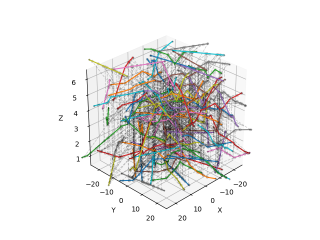
# Figure
fig, ax = plt.subplots(subplot_kw=dict(projection='3d', aspect='equal',
                                       xlabel="X", ylabel="Y", zlabel="Z"))
ax.view_init(azim=45, elev=30, roll=0)
if len(mesh):
    # Draw elements
    for i, j, k in tqdm(zip(mesh.index, mesh.beam, mesh.constraint),
                        total=len(mesh), desc="Draw mesh"):
        # Get element data
        a, b, c = mesh.iloc[[i, j, k]][[*"xyz"]].values
        if mesh.iloc[i].s < mesh.iloc[j].s:
            # Draw intra-fiber connection
            plt.plot(*np.c_[a, b],
                     c=plt.cm.tab10(mesh.fiber.iloc[i] % 10))
        if mesh.iloc[i].z < mesh.iloc[k].z:
            # Draw inter-fiber connection
            plt.plot(*np.c_[a, c], '--ok',
                     lw=1, mfc='none', ms=3, alpha=0.2)
        if mesh.iloc[i].fiber == mesh.iloc[k].fiber:
            # Draw fiber end nodes
            plt.plot(*np.c_[a, c], '+k', ms=3, alpha=0.2)
# Set drawing box dimensions
ax.set_xlim(-0.5 * mesh.attrs["size"], 0.5 * mesh.attrs["size"])
ax.set_ylim(-0.5 * mesh.attrs["size"], 0.5 * mesh.attrs["size"])
plt.show()